DensityFunction

The DensityFunction algorithm provides a consistent and streamlined workflow to create and store density functions and utilize them for anomaly detection. DensityFunction allows for grouping of the data using the by clause, where for each group a separate density function is fitted and stored. This algorithm supports partial_fit.

Note: For more information on using the by clause see the Syntax constraints section.

The DensityFunction algorithm supports the following continuous probability density functions: Normal, Exponential, Gaussian Kernel Density Estimation (Gaussian KDE), and Beta distribution.

Note: Using the DensityFunction algorithm requires running the latest version of the Python for Scientific Computing (PSC) add-on, for example version 3.2.4.

The accuracy of the anomaly detection for DensityFunction depends on the quality and the size of the training dataset, how accurately the fitted distribution models the underlying process that generates the data, and the value chosen for the threshold parameter.

To learn more about the DensityFunction algorithm in the AI Toolkit see Using the DensityFunction algorithm in the Splunk Machine Learning Toolkit.

Follow these guidelines to make your models perform more accurately:

• For best results use at least 50 data points when fitting a distribution. Avoid using fields with very low cardinality (few unique values), as they do not produce meaningful density estimates.

  • If additional data is not available, consider reducing the number of groups created with the by clause so that each group contains more data points.`

• The threshold parameter has a default value, but ideally the value for threshold, lower_threshold, or upper_threshold are chosen based on experimentation as guided by domain knowledge.

• Continue tuning the threshold parameter until you are satisfied with the results.

• Inspect the model using the summary command.

  • The values reported for the mean and standard deviation are either the statistics of the fitted distribution, or of the data, depending on the type of the distribution.
  • In the case of parametric distributions (Normal, Beta, and Exponential) the mean and standard deviation are calculated from the fitted distribution. When the parametric distribution is not a good fit for the data, the reported mean and std might not be close to that of data.
  • In the case of non-parametric distributions (Gaussian KDE) the mean and standard deviation are calculated from the data passed in during fit.

• If the distribution of the data changes through time, re-train your models frequently.

Parameters

• The partial_fit parameter controls whether an existing model should be incrementally updated or not. This allows you to update an existing model using only new data without having to retrain it on the full training data set.

  • The partial_fit parameter default is False.
  • If partial_fit is not specified, the model specified is created and replaces the pre-trained model if none exists.

• Using partial_fit=True on an existing model ignores the newly supplied parameters. The parameters supplied at model creation are used instead.

• The supervise_split_by parameter is available with MLTK version 5.5.0 or higher and this parameter can be set to true or false.

  • When set to true, the fields entered in the by clause are used by a decision tree algorithm to automatically generate groups in the dataset

• Valid values for the dist parameter include: norm (normal distribution), expon (exponential distribution), gaussian_kde (Gaussian KDE distribution), beta (beta distribution), and auto (automatic selection).

  • The dist parameter default is auto.
  • When set to auto, norm (normal distribution), expon (exponential distribution), gaussian_kde (Gaussian KDE distribution) , and beta (beta distribution) all run, with the best results returned.

• Use the exclude_dist parameter to exclude a minimum of 1 and a maximum of 3 of the available dist parameter values (norm, expon, gaussian_kde, beta).

  • The exclude_dist parameter is only available when the dist parameter is auto.
  • DensityFunction will run using any non-excluded dist parameter values.
  • Use a comma to note multiple excluded dist parameter values. For example, exclude_dist="beta,expon"
  • Attempts to use the exclude_dist parameter on more than 3 dist parameter values, or on a dist parameter other than auto will result in an error message.

• Beta distribution was added in version 5.2.0 of the Machine Learning Toolkit

  • If the data distribution takes a U shape, outlier detection will not be accurate.

• The metric parameter calculates the distance between the sampled dataset from the density function and the training dataset.

• Valid metrics for the metric parameter include: kolmogorov_smirnov and wasserstein.

• The metric parameter default is wasserstein.

• The sample parameter can be used during fit or apply stages.

• The sample parameter default is False.

• If the sample parameter is set to True during the fit stage, the size of the samples will be equal to the training dataset.

• If the sample parameter is set to True during the apply stage, the size of the samples will be equal to the testing dataset.

• If the sample parameter is set to True:

  • Samples are taken from the fitted density function.
  • Results output in a new column called SampledValue.
  • Sampled values only come from the inlier region of the distribution.

• The full_sample parameter can be used during fit or apply stages.

• The full_sample parameter default is False.

• If the full_sample parameter is set to True during the fit stage, the size of the samples will be equal to the training dataset.

• If the full_sample parameter is set to True during the apply stage, the size of the samples will be equal to the testing dataset.

• If the full_sample parameter is set to True:

  • Samples are taken from the fitted density function.
  • Results output in a new column called FullSampledValue.
  • Sampled values come from the whole distribution (both inlier and outlier regions).

• Use the summary command to inspect the model.

  • The values reported for the mean and standard deviation are either the statistics of the fitted distribution, or of the data, depending on the type of the distribution.
  • In the case of parametric distributions (Normal, Beta, and Exponential) the mean and standard deviation are calculated from the fitted distribution. When the parametric distribution is not a good fit for the data, the reported mean and std might not be close to that of data.
  • In the case of non-parametric distributions (Gaussian KDE) the mean and standard deviation are calculated from the data passed in during fit.

• Version 4.4.0 and higher of MLTK support min and max values in summary.

  • The min value is the minimum value of the dataset on which the density function is fitted.
  • The max value is the maximum value of the dataset on which the density function is fitted.

• The cardinality value generated by the summary command represents the number of data points used when fitting the selected density function.

• The distance value generated by the summary command represents the metric type used when calculating the distance as well as the distance between the sampled data points from the density function and the training dataset.

• The mean value generated by the summary command is the mean of the density function.

• The value for std generated by the summary command represents the standard deviation of the density function.

• A value under other represents any parameters other than mean and std as applicable. In the case of Gaussian KDE, other could show parameter size or bandwidth.

• The type field generated by the summary command shows both the chosen density function as well as if the dist parameter is set to auto.

• The show_density parameter default is False. If the parameter is set to True, the density of each data point will be provided as output in a new field called ProbabilityDensity.

• The output for ProbabilityDensity is the probability density of the data point according to the fitted probability density. This output is provided when the show_density parameter is set to True.

• The fit command will fit a probability density function over the data, optionally store the resulting distribution's parameters in a model file, and output the outlier in a new field called IsOutlier.

• The output for IsOutlier is a list of labels. Number 1 represents outliers, and 0 represents inliers, assigned to each data point. Outliers are detected based on the values set for the threshold parameter. Inspect the IsOutlier results column to see how well the outlier detection is performing.

• The parameters threshold, lower_threshold, and upper_threshold control the outlier detection process.

• The threshold parameter is the basis of the outlier detection process. It represents the percentage of the area under the density function and has a value between 0.000000001 (refers to ~0%) and 1 (refers to 100%). The threshold parameter guides the DensityFunction algorithm to mark outlier areas on the fitted distribution. For example, if threshold=0.01, then 1% of the fitted density function will be set as the outlier area.

• The threshold parameter default value is 0.01.

• The threshold, lower_threshold, and upper_threshold parameters can take multiple values. Multiple values must be in quotation marks and separated by commas as shown in the following example:

| tstats count where index=web by client_ip
| rename count AS requests
| fit DensityFunction requests by client_ip into requests_density_by_ip threshold="0.01,0.05,0.1"

• In cases of multiple values for threshold, the default maximum is 5. Users with access permissions can change this default maximum under the Settings tab.

  • In cases of multiple values, you are limited to one type of threshold (threshold,lower_threshold, or upper_threshold).

• The output for BoundaryRanges is the boundary ranges of outliers on the density function which are set according to the values of the threshold parameter.

• Each boundary region has three values: boundary opening point, boundary closing point, and percentage of boundary region.

• The boundary region syntax follows the convention of a multi-value field where each boundary region appears in a new line:

first_boundary_region
second_boundary_region
n_th_boundary_region

• When multiple thresholds are provided, Boundary Ranges for each threshold appears in a different column separated with the suffix of _th=and the threshold values:

BoundaryRanges_th=threshold_val_1
first_boundary_region_of_th1
second_boundary_region_of_th1
n_th_boundary_region_of_th1

BoundaryRanges_th=threshold_val_2
first_boundary_region_of_th2
second_boundary_region_of_th2
n_th_boundary_region_of_th2

• In cases of a single boundary region, the value for the percentage of boundary region is equal to the threshold parameter value.

• In some distributions (for example Gaussian KDE), the sum of outlier areas might not add up to the exact value of threshold parameter value, but will be a close approximation.

• BoundaryRangesis calculated as an approximation and will be empty in the following two cases:

  • Where the density function has a sharp peak from low standard deviation.
  • When there are a low number of data points.

• Data points that are exactly at the boundary opening or closing point are assigned as inliers. An opening or closing point is determined by the density function in use.

• Normal density function has left and right boundary regions. Data points on the left of the left boundary closing point, and data points on the right of the right boundary opening point are assigned as outliers.

• Exponential density function has one boundary region. Data points on the right of the right boundary opening point are assigned as outliers.

• Beta density function has one boundary region. Data points on the left of the left boundary closing point are assigned as outliers.

• Gaussian KDE density function can have one or more boundary regions, depending on the number of peaks and valleys within the density function. Data points in these boundary regions are assigned as outliers. In cases of boundary regions to the left or right, guidelines from Normal density function apply. As the shape for Gaussian KDE density function can differ from dataset to dataset, you do not consistently observe left and right boundary regions.

• The random_state parameter is the seed of the pseudo random number generator to use when creating the model.

  • This parameter is optional but the value must be an integer.

  • The random_state default is value is None.

  • When parameter value is None, the split is randomized.

  • When parameter value is an integer, the reproducible random sampling uses the specified seed.

• The show_options="feature_variables, split_by, params" parameter in the DensityFunction algorithm is used to prepare the data for display using the Distribution Plot. See the following for details about the model's configuration:

  • feature_variables: This option displays the names of the fields that the DensityFunction algorithm used to build the density model. These are the fields specified in the <field> parameter of the fit DensityFunction command.
  • split_by: If you use a by clause in your fit DensityFunction command, such as by "shop_id". This option displays the fields used for grouping the data. The DensityFunction algorithm fits a separate density function for each group defined by these fields.
  • params: This option displays the parameters that were used when fitting the DensityFunction model. This can include parameters like dist (distribution type) and threshold, which are crucial for understanding how the model identifies outliers.

• When you include these show_options configurations in the fit DensityFunction command, along with show_density=True, you can visualize the results using the Distribution Plot.

• The following command fits a density function to the quantity field, grouped by shop_id, using an automatic distribution and a threshold of 0.01. The show_options argument ensures that the Distribution Plot displays the feature variable (quantity), the split-by field (shop_id), and the parameters used in the model such as dist=auto, threshold=0.01:

| fit DensityFunction "quantity" by "shop_id" dist=auto threshold=0.01 show_density=True show_options="feature_variables,split_by,params"

Syntax

| fit DensityFunction <field> [by "<field1>[,<field2>,....<field5>]"] [into <model name>] [dist=<str>] [show_density=true|false] [sample=true|false][full_sample=true|false][threshold=<float>|lower_threshold=<float>|upper_threshold=<float>] [metric=<str>] [random_state=<int>] [partial_fit=<true|false>]

You can apply the saved model to new data with the apply command, with the option to update the parameters for threshold, lower_threshold, upper_threshold, and show_density. Parameters for dist and metric cannot be applied at this stage, and any new values provided will be ignored.

apply <model name> [threshold=<float>|lower_threshold=<float>|upper_threshold=<float>] [show_density=true|false][sample=true|false][full_sample=true|false]

You can inspect the model learned by DensityFunction with the summary command. Version 4.4.0 or higher of MLTK supports min and max values in the summary command.

| summary <model name>

Syntax constraints

• Fields within the by clause must be given in quotation marks.

• The maximum number of fields within the by clause is 5.

• The total number of groups calculated with the by clause can not exceed 1024. In an example clause of by "DayOfWeek,HourOfDay" there are two fields: one for DayOfWeek and one for HourOfDay. As there are seven days in a week, there are seven groups for DayOfWeek. As there are twenty-four hours in a day, there are twenty-four groups for HourOfDay. Meaning the total number of groups calculated with the by clause is 7*24= 168.

  • The limited number of groups prevents model files from growing too large. You can increase the limit by changing the value of max_groups in the DensityFunction settings. Larger limits mean larger model files and longer load times when running apply.
  • Decrease max_kde_parameter_size to allow for the increase of max_groups. This change keeps model sizes small while allowing for increased groups.

• Field names used within the by clause that match any one of the reserved summary field names, produces an error. You must rename your field(s) used within the by clause to fix the error. Reserved summary field names include: type, min, max, mean, std, cardinality, distance, and other.

• The parameters threshold, lower_threshold, and upper_threshold must be within the range of 0.00000001 to 1.

• If the parameters of lower_threshold and upper_threshold are both provided, the summation of these parameters must be less than 1 (100%).

• The threshold and lower_threshold / upper_threshold parameters can not be specified together.

• The threshold, lower_threshold, and upper_threshold parameters can take multiple values but in these cases you are limited to one type of threshold (threshold,lower_threshold, or upper_threshold).

• Exponential density function only supports threshold and upper_threshold.

• Exponential density function supports using lower_threshold but results in empty Boundary regions and 0 outliers.

• Normal density function supports either threshold or lower_threshold / upper_threshold.

• Gaussian KDE density function supports either threshold or lower_threshold / upper_threshold.

• The parameters lower_threshold and upper_threshold can be used with any density function including auto.

  • Exponential density function supports using lower_threshold but results in empty Boundary regions and 0 outliers.

• If you use the summary command to inspect a model created in version 4.3.0 or lower of MLTK (prior to the support of min and max), approximate values for min and max are used.

Examples

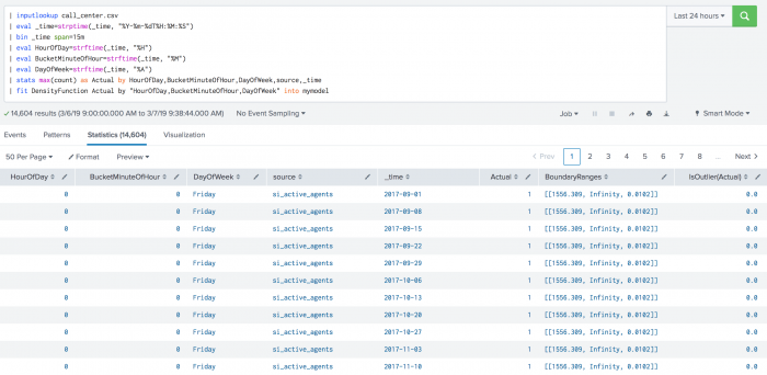
The following example shows DensityFunction on a dataset with the fit command.

| inputlookup call_center.csv
| eval _time=strptime(_time, "%Y-%m-%dT%H:%M:%S")
| bin _time span=15m
| eval HourOfDay=strftime(_time, "%H")
| eval BucketMinuteOfHour=strftime(_time, "%M")
| eval DayOfWeek=strftime(_time, "%A")
| stats max(count) as Actual by HourOfDay,BucketMinuteOfHour,DayOfWeek,source,_time
| fit DensityFunction Actual by "HourOfDay,BucketMinuteOfHour,DayOfWeek" into mymodel

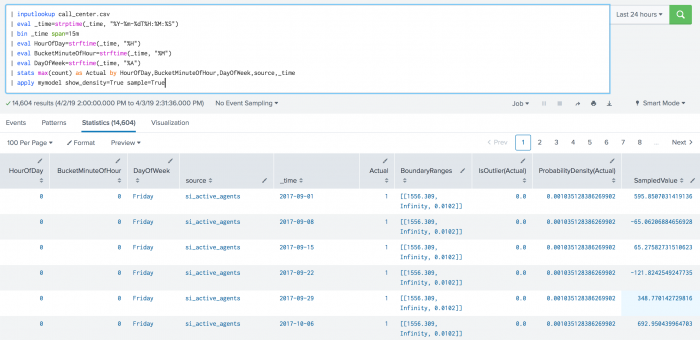
The following example shows DensityFunction on a dataset with the apply command.

| inputlookup call_center.csv
| eval _time=strptime(_time, "%Y-%m-%dT%H:%M:%S")
| bin _time span=15m
| eval HourOfDay=strftime(_time, "%H")
| eval BucketMinuteOfHour=strftime(_time, "%M")
| eval DayOfWeek=strftime(_time, "%A")
| stats max(count) as Actual by HourOfDay,BucketMinuteOfHour,DayOfWeek,source,_time
| apply mymodel show_density=True sample=True

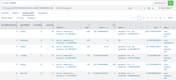
The following example shows DensityFunction on a dataset with the summary command. This example includes min and max values, which are supported in version 4.4.0 and higher of MLTK.

| summary mymodel

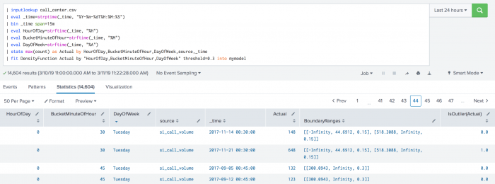
The following example shows BoundaryRages on a test set. In this example the threshold is set to 30% (0.3). The first row has a left boundary range which starts at -Infinity and goes up to the number 44.6912. The area of the left boundary range is 15% of the total area under the density function. It has also a right boundary range which starts at a number 518.3088 and goes up to Infinity. Again, the area of the right boundary range is the same as the left boundary range with 15% of the total area under the density function. The areas of right and left boundary ranges add up to the threshold value of 30%. The third row has only one boundary range which starts at number 300.0943 and goes up to Infinity. The area of the boundary range is 30% of the area under the density function.

| inputlookup call_center.csv
| eval _time=strptime(_time, "%Y-%m-%dT%H:%M:%S")
| bin _time span=15m
| eval HourOfDay=strftime(_time, "%H")
| eval BucketMinuteOfHour=strftime(_time, "%M")
| eval DayOfWeek=strftime(_time, "%A")
| stats max(count) as Actual by HourOfDay, BucketMinuteOfHour, DayOfWeek, source, _time
| fit DensityFunction Actual by "HourOfDay, BucketMinuteOfHour, DayOfWeek" threshold=0.3 into mymodel

Local availability Permalink to this section#

• Local class: DensityFunction
• Source file: Splunk_ML_Toolkit/bin/algos/DensityFunction.py (in-repo path Splunk_ML_Toolkit/bin/algos/DensityFunction.py)
• algos.conf stanza: [DensityFunction]
• Class bases: BaseAlgo

Source Permalink to this section#

Adapted from the Splunk AI Toolkit 5.6.4 documentation at /en/splunk-cloud-platform/apply-machine-learning/use-ai-toolkit/5.6.4/algorithms-and-scoring-metrics-in-the-ai-toolkit/algorithms-in-the-ai-toolkit (section: anomaly).